Bootstrapping a Poisson GLMM with glmmBoot
This code to illustrates the implementation of the bootstrapping methods described in (Flores-Agreda and Cantoni, Under Review) in a real-data context. Data comes from the example found in Molenberghs & Verbeke (2006) initially reported by Faught et. al. (1996).
Analysis
To start performing the analysis, you need:
- the following packages:
library(lme4)
library(glmmTMB)
library(sas7bdat)
library(TMB)
library(dplyr)
library(ggplot2)- to compile
glmm_rirs.cppand load the resulting binary into the environment:
compile(file = "glmmBoot/src/glmm_rirs.cpp")
dyn.load(dynlib("glmmBoot/src/glmm_rirs"))- the functions in the file
glmmBoot.R:
source("glmmBoot/R/glmmBoot.R")- the dataset
epilepsy.sas7bdat
epilepsy <- read.sas7bdat(file = "glmmBoot/data/epilepsy.sas7bdat")Model
The aim of the study was to verify the effects of an new anti-epileptic drug (AED) compared to a placebo on the number of seizures experienced by patients during the study. To do this, consider a mixed Poisson model for the outcome containing two potentially correlated random effects: one for a random intercept and another one for the visit time i.e. \(y_{ij}|\mathbf{u}_i\sim \mathcal{P}(\lambda_{ij})\) with:
\[\log(\lambda_{ij}) = \beta_0 + \beta_{1} T_{ij} + \beta_{2}t_{ij} + \beta_{3} T_{ij}t_{ij} + \sigma_{1} u_{i1} + \sigma_{2} u_{i2} t_{ij}\]
where:
- \(T_{ij}\) represents the effect of the treatment and
- \(t_{ij}\) the visit time.
The variance-covariance structure of the vector of Normal random effects \(\mathbf{u}_i = [u_{i1}, u_{i2}]^T\), comprises a correlation coefficient \(\rho\) , i.e.
\[\mathbf{D}(\mathbf{\sigma}) = \left[\begin{array}{c c} \sigma_{1}^2 & \rho\sigma_{1}\sigma_{2} \\ \rho\sigma_{1}\sigma_{2} & \sigma_{2}^2 \end{array}\right].\]
Implementation
estimate_glmm()
The function estimate_glmm() estimates the model with a TMB template using the frame and estimates of objects of class glmerMod as starting values. For example:
obj.glmerMod <- lme4::glmer(nseizw~ trt*studyweek + (studyweek|id),
                            family = "poisson",
                            data = epilepsy,
                            control = glmerControl(optimizer = "bobyqa"))
for comparison purposes, let us also extract the estimates of this object
A comparison of the estimates yields:
est_lmer %>%
  inner_join(est_tmb, by=("Parameters"), suffix=c(" (glmer)", " (TMB)")) %>%
kable(digits = 4)| Parameters | Estimates (glmer) | Std..Errors (glmer) | Estimates (TMB) | Std..Errors (TMB) |
|---|---|---|---|---|
| (Intercept) | 0.8945 | 0.1782 | 0.8945 | 0.1786 |
| trt | -0.2443 | 0.2538 | -0.2443 | 0.2544 |
| studyweek | -0.0271 | 0.0099 | -0.0271 | 0.0099 |
| trt:studyweek | 0.0107 | 0.0138 | 0.0107 | 0.0139 |
| s_1 | 1.1272 | NA | 1.1273 | 0.0975 |
| s_2 | 0.0487 | NA | 0.0487 | 0.0057 |
| rho | -0.3339 | NA | -0.3339 | 0.1312 |
The generation of replicates using Random Weighted Laplace Bootstrap (Flores-Agreda and Cantoni, Under Review) is carried by the function bootstrap_glmm(), with the option method=rwlb.
## Bootstrap inference
rwlb_reps <- bootstrap_glmm(obj.glmerMod,
                            B = 1000,
                            method = "rwlb")
The resulting Bootstrap replicates are stored in an object of the class glmmBoot, which can be used to construct:
- Estimates of the Parameters: by averaging over the replicates.
- Estimates of the Standard Errors: by computing the standard deviations for the replicates.
- Percentile-based and Studentized Confidence Intervals (CI) with a level of 95%.
Methods
confint()
produces bootstrap estimates, standard errors and confidence intervals with the percentile and studentized methods
- Example of the percentile method
rwlb_reps %>%
  confint(bootstrap_type = "percentile")%>%
kable(digits = 4)| Parameters | Estimate | Std_Errors | ci_lower | ci_upper |
|---|---|---|---|---|
| (Intercept) | 0.8890 | 0.1550 | 0.5771 | 1.1726 |
| rho | -0.3193 | 0.1623 | -0.6379 | -0.0232 |
| s_1 | 1.1068 | 0.1288 | 0.8879 | 1.3936 |
| s_2 | 0.0471 | 0.0073 | 0.0335 | 0.0625 |
| studyweek | -0.0271 | 0.0087 | -0.0449 | -0.0113 |
| trt | -0.2372 | 0.2512 | -0.7172 | 0.2332 |
| trt:studyweek | 0.0106 | 0.0139 | -0.0164 | 0.0375 |
- Example of the studentized method
rwlb_reps %>%
  confint(bootstrap_type = "studentized") %>%
kable(digits = 4)| Parameters | Estimate | Std_Errors | ci_lower | ci_upper |
|---|---|---|---|---|
| (Intercept) | 0.8890 | 0.1550 | 0.5820 | 1.1882 |
| rho | -0.3193 | 0.1623 | -0.7402 | -0.0651 |
| s_1 | 1.1068 | 0.1288 | 0.8292 | 1.3248 |
| s_2 | 0.0471 | 0.0073 | 0.0316 | 0.0601 |
| studyweek | -0.0271 | 0.0087 | -0.0446 | -0.0099 |
| trt | -0.2372 | 0.2512 | -0.7369 | 0.2429 |
| trt:studyweek | 0.0106 | 0.0139 | -0.0163 | 0.0374 |
plot()
Shows the boxplots of the replicates for all the parameters or a subset with a line describing the TMB estimates
- fixed effect parameters
plot(rwlb_reps,
     parm_subset=c("(Intercept)", "trt", "studyweek", "trt:studyweek")) +
  ggtitle("Replicates of Fixed Effects") +
  theme_classic()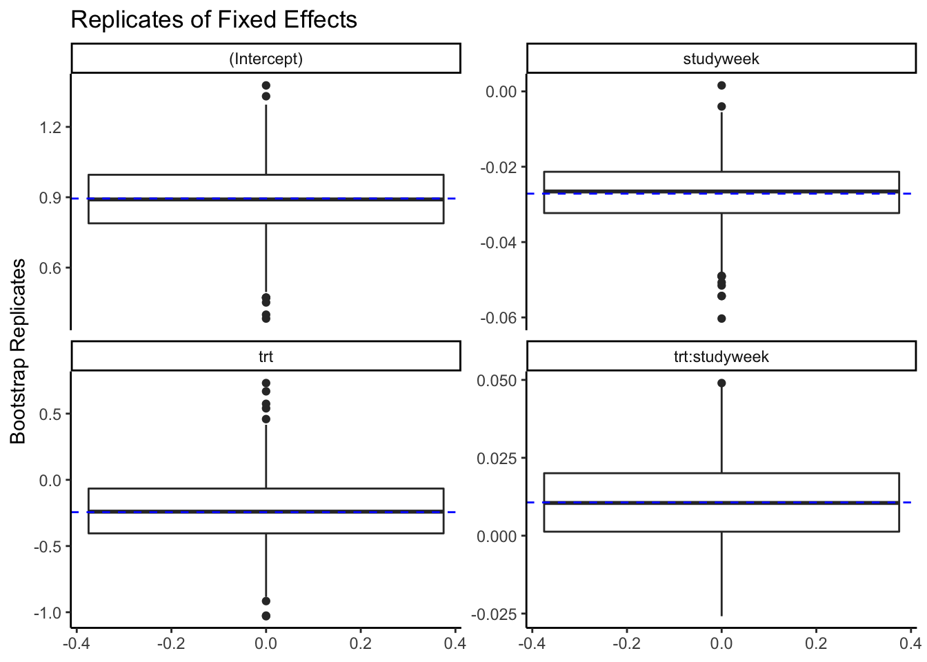
- variances of random effects
plot(rwlb_reps,
     parm_subset=c("s_1", "s_2", "rho")) +
  ggtitle("Replicates of Variance Components")+
  theme_classic()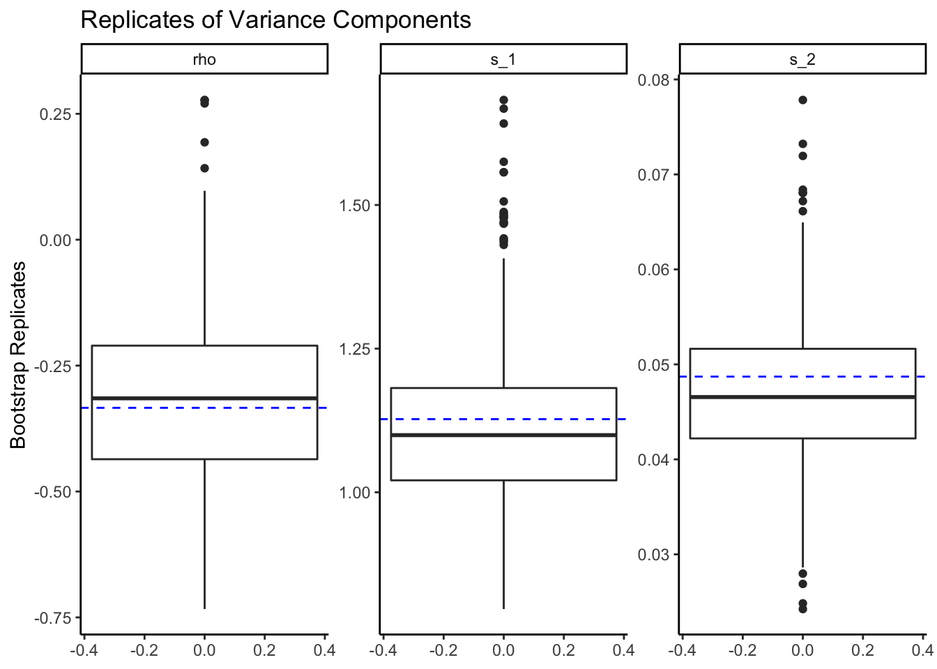
Daniel Flores-Agreda
Research Fellow (Biostatistics)
School of Public Health and Preventive Medicine of Monash University.